Higgs Hunting in Uppsala

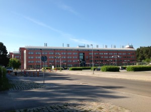
The Angstrom Laboratory
The Angstrom Laboratory. Only 1/6 of the complex is visible in this photo. It is home to many branches of science, including physics.

Two days ago, I arrived in Uppsala, Sweden, so that I could spend a day working and interacting with the ATLAS group at the University of Uppsala (Uppsala Universitet). Uppsala is a beautiful city located north of Stockholm, just a short bus ride from the Stockholm Arlanda Airport (where I landed). Everything in Uppsala is within comfortable walking distances (~30 minutes in any direction), and the city has a wonderful mix of history and modernity. Uppsala may be one of my favorite places on Earth, and to boot ATLAS group here is a powerhouse in physics that is very interesting to me.

I’ve talked about the charged Higgs boson before – the subatomic chimera that wears both the spin and couplings of a Higgs boson and also the electric charge that denotes a coupling via the electromagnetic interaction. This unique beast is not of the Standard Model, but appears automatically in even modest extensions of the Standard Model. Such extensions are needed to explain how particles outside the Standard Model, such as dark matter, acquire their mass. If the Higgs mechanism is the way in which nature gives mass to particles, then there is an excellent chance that the charged Higgs exists in nature. Only by careful experimentation can we know.
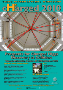
Poster from CHARGED-2010, the last installment of the Uppsala-hosted charged Higgs boson conference.

The Uppsala group has rich history of investigation into the charged Higgs boson, and routinely hosts a conference on the subject (every two years, typically in September). Yesterday, they were gracious enough to host me in their department. I even attended their Friday morning meeting, where they discussed the latest updates on their research (some of which is aimed for the ICHEP conference in a few weeks). They even set aside time at the end for a discussion with me about plans to extend the search for the charged Higgs boson beyond its current confines, taking advantage of the unique strengths of the Large Hadron Collider to define a new front in the search for this particle.

Having only arrived in Europe on Wednesday morning, and being in the throes of jet lag, being able to interact with the students and faculty of the Uppsala group has energized me. I’ve also had the chance to spend a little time in Uppsala itself, having lunch with some of the Ph.D. students by the river and walking the streets to find new sites I have not yet seen (and getting my exercise in the process).

Below are some of the photos that I shot while on my wanderings around Uppsala. One of my favorite parts of the city is the Domkyrkan (cathedral), which one of the students quipped probably took longer to build than the U.S. is old. I love it that, in Europe, you can readily find examples of such things that set the youth of my home nation in perspective.

[nggallery id=3]

Python and ROOT Tricks: efficiency graphs

You are asked to produce a graph showing the efficiency of selecting a sample as a function of a variable. Let’s called that variable x. How do you do this with PyROOT, and how do you make sure (most importantly) that the errors associated with each point in the efficiency graph are correct?

The underlying trap is a simple one. You are immediately tempted to produce two histograms showing the distribution of variable x. One of them shows the distribution before your selection, and the other shows the distribution after your selection. You then use the native ROOT “TH1::Divide()” method of the histogram class to make the efficiency graph. For instance:

h_before_selection = ROOT.TH1F("h_before_selection","",100,0,10)
h_before_selection.Sumw2()
h_after_selection = ROOT.TH1F("h_after_selection","",100,0,10)
h_after_selection.Sumw2()
# do something that fills the histograms with the right events
# ... more code here ...
# now divide them to make an efficiency histogram
h_efficiency = h_after_selection
h_efficiency.Divide(h_before_selection)

So, does this work? Well, it will certainly produce a histogram showing the efficiency as a function of the variable. But what about the errors? They will be very wrong.

Why are the errors incorrect? When you call the default TH1::Divide method, it assumes the data in the two histograms are uncorrelated. But we know that the histogram after selection contains a subset of the events in the histogram before selection, making them correlated. This is exactly the situation handled by binomial errors, where you have two categories into which events can be placed – selected or unselected – and those errors define an exact prescription for correct computation.

ROOT provides a version of TH1::Divide that does this treatment correctly. Here is how you do it:

h_efficiency = h_after_selection
h_efficiency.Divide(h_after_selection,h_before_selection,1.0,1.0,"B")

This divides the two histograms (multiplying each of them first by a factor of 1.0) and computes the binomial errors in each bin of the histogram.

Now, there is one thing here that might annoy some people: when a bin retains all events from prior to the selection, the efficiency is 100% and the binomial prescription yields an error of 0% on that bin. However, some of you may wish to take into account the fact that you know that bin contains a finite statistics and there is some uncertainty on the efficiency as a result. How do you handle this?

The TGraphAsymmErrors class comes to the rescue. It defines a Divide() method (in the very latest version of ROOT; in versions prior to 5.28, you have to call TGraphAsymmErrors::BayesDivide()) that will take into account the finite statistics of a bin with 100% efficiency, using a Bayesian Prior to compute a lower error (the upper error is still 0%, of course). To use this:

g_efficiency = ROOT.TGraphAsymmErrors()
g_efficiency.Divide(h_after_selection,h_before_selection,"cl=0.683 b(1,1) mode")

For versions of ROOT prior to 5.28, use instead:

g_efficiency.BayesDivide(h_after_selection,h_before_selection)

There are more options available for the TGraphErrors::Divide method. Check out the class documentation for more information, and enjoy your new-found prowess with histograms and errors!

References:

http://root.cern.ch/root/html/src/TGraphAsymmErrors.cxx.html#CBi_IC

http://root.cern.ch/root/html/src/TGraphAsymmErrors.cxx.html#G9MXkE

http://root.cern.ch/root/html/TH1.html#TH1:Divide%1

Python and ROOT Tricks: vectors of vectors

Many thanks to Matt Bellis for this tip!

You can write very complex objects to a ROOT TTree. For instance, you might encounter a TBranch in a TTree that is of type

std::vector< std::vector<float> >

This is a C++ STL vector object nested inside another such object. How do you handle this in Python?

The trick, outlined below, may or may not work with your particular combination of ROOT and Python. For instance, when I tried this with ROOT 5.26.00e and Python 2.4 (the default combination in Scientific Linux 5), I got all kinds of errors. When I switched to 5.28 and Python 2.4 or 2.7, it worked great. So, your mileage may vary.

Here is the trick. You need to tell Python and ROOT how to handle such TBranch types. To do this, you need to write an external ROOT C++ macro which can be loaded and compiled by CINT; this then directs ROOT on just what is a vector of a vector. Here is the macro:

// stl_loader.h
#include<vector>

#ifdef __CINT__
#pragma link C++ class vector<vector<float> >;
#else
template class std::vector<std::vector<float> >;
#endif

Now you need to have your Python program load and compile this file into a library at the very beginning of the program:

import ROOT
ROOT.gROOT.LoadMacro("load_stl.h+")

Now you can access the vector of vectors in your code as follows:

// Assume the TBranch in your TTree is called "VecOfVecFloat"
TheVectorOfVectors = aTree.VecOfVecFloat
print len(TheVectorOfVectors)
if len(TheVectorOfVectors) > 0:
    VectorOfFloats = TheVectorOfVectors[0]
    print len(VectorOfFloats)
    if len(VectorOfFloats) > 0:
        aFloat = VectorOfFloats[0]
        print aFloat

Now you should be able to use those floats buried in a vector buried inside another vector. Good luck!