
It has been 73 days since Texas, racing to reopen without first putting in place large-scale testing and tracing infrastructure, ceded the population of the state to the SARS-CoV-2 virus. That was COVID Day, or C-Day: May 1, 2020.
On C-Day, Texas announced that businesses could re-open at 25% capacity; however, it did so without first preparing for the consequences. The reopening march proceeded then on a schedule driven, not by data and epidemiology, but by arbitrary mandates from the governor about when the next phase of opening should occur. Seven days after the first step, salons were allowed to reopen. This was despite the fact that if the first step causes new cases in the community, they would not show up for 14-21 days after the step; 7 days was just too soon to tell, and thus to move to the next step. That is what is meant by “reopening too fast” – taking the next step before the last one’s effects can be measured.
The data did tell an interesting story, though, which I will get to later. The summary of all of this is that my county, Collin County, has (like most urban parts of Texas) experienced slow, then rapid, growth in the spread of SARS-CoV-2. The data suggest that transmission started almost immediately as Texas began its reopening. Some factors might have contributed to faster and more rapid spread of the virus.
Under the hood, at each choice, there is the slow burn of normal exponential growth mathematics. If the doubling time for a process is 20 days, then you will see small growth in the first 20 days; in the next 20 days, the number will double again; 20 days later, it will double again. What you might attribute at first to “normal growth” may, in fact, be the first signs of out-of-control exponential growth. Having enough data to tell the difference is the key to avoiding resurgence of a communicable disease.

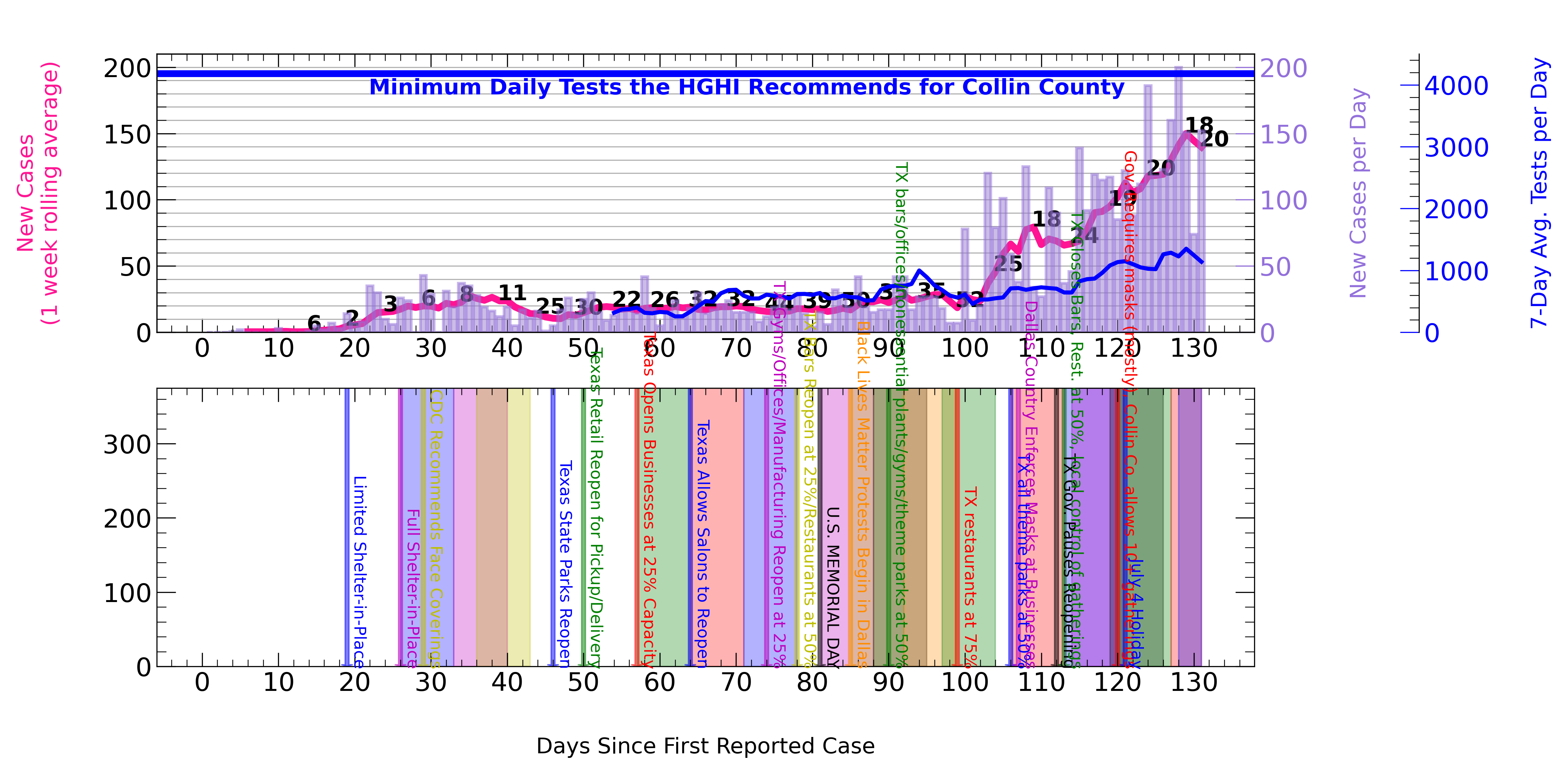
Bottom Graph: Vertical color lines indicate key events in Texas and Collin County, such as shelter-in-place orders or reopening stages; colored bands, 7-14 days after the color line, indicate the range of expected effects in the data. However, current evidence suggests the more accurate window may be 14-21 days after an event that can alter the pandemic’s course.
The above graph tells the tale of new cases per day. Those have skyrocketed in the last month, from about 25 per day in May to over 100 per day in June and now July.
Let’s pause for a moment and think about the math of exponential growth. If something is growing exponentially at a constant rate (e.g. a fixed doubling rate of, say, 20 days), then after every unit of 20 days the process has to yield more growth per day to maintain the rate. Exponential growth demands an increase, with time, of the appearance of new things each day. For example, let’s say that on day 0 you have 10 cases. At a doubling rate of 20 days, then 20 days later you will have 20 cases. On average, you added 0.5 cases per day during the first 20 days. On day 40, you expect to have 40 cases – twice what you had on day 20. From day 20 to day 40, you are now adding 1 case per day, on average – a higher rate of cases per day than in the first twenty days. On day 60, you expect to have 80 cases total … that is an average new-case rate of 2 cases per day during the third 20-day period.
In each new period of 20 days, you add more cases per day to maintain the 20-day doubling rate. That’s the demand of exponential growth.
So if you are dealing with a disease, and you add 25 cases per day for the first 20 days, then also again during the next 20 days, you are out of the realm of exponential growth. You won’t double the number of cases every 20 days; at a constant rate of adding new cases, it will take longer, and longer, and longer to double the total number of cases. That would be more of a sign that you have established a measure of control over the spread.
Which brings me to a bit of data analysis fun. I decided to employ a very basic strategy to understand whether or not certain choices made the spread of SARS-CoV-2 worse or better in Collin County. These are NOT the conclusions of an epidemiologist, and should not be substituted for input from actual experts in disease modeling (UT Southwestern, a premiere medical institution in Dallas, has an EXCELLENT model you should all pay attention to [1]). However, I think there is some useful information in this very primitive analysis.
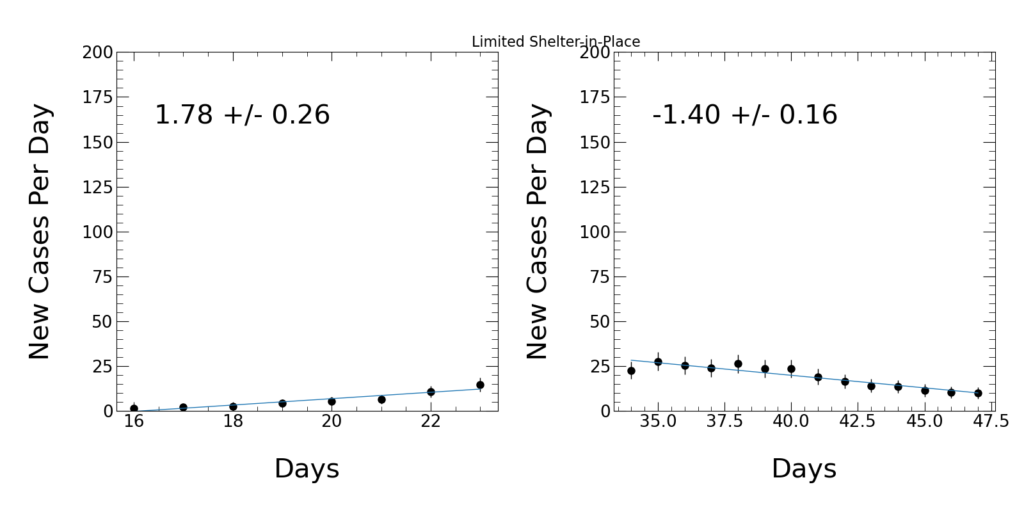
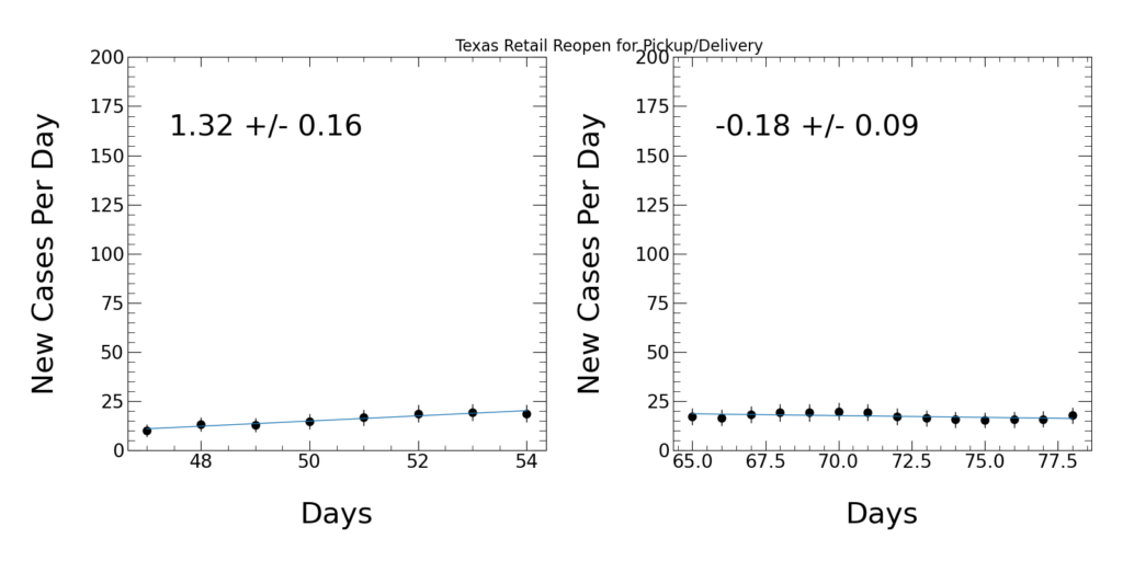
Here is the idea. Pick an event, like the limited shelter-in-place order put in place in Collin County on March 24, 2020. Put a window in time around that event, and fit the number of new cases per days using a simple linear model, y = mx + b (where y is the number of cases per day, x is the day, m is the slope, and b is the y-intercept). I used a window of 3 days on either side, centered on the day of the event. This provides a measure of how the disease was spreading (the slope of the new cases per day) at the time of the event.
Then slide 14-21 days layer. By this time, the effects of the event from earlier would have begun to show up in the case counts, according to the current understanding of the infection rate, symptom emergence, and testing time. In that time window 14-21 days later, again fit a straight line and get the slope.
Most importantly, get the uncertainty on the slopes from the two linear fits, which is determined from the fitting procedure.
I then use a simple numerical measure of the impact:
- If the original slope was positive, and the later slope is negative, then this appears to be a “positive reversal” of the original trend (things were getting worse and now they are getting better).
- If the original slope was negative, and the later slope is positive, then this appears to a “negative reversal” of the original trend (things were going in the right direction, then got worse later, reversing the original improvement)
- If the later slope is greater (less) than the original one, then things got worse (better).
The difference in the two slopes, subtracting the later slope from the original, is a measure of their similarity. The closer to zero the difference of the two numbers, the more similar the two periods are. The total uncertainty on the difference is the sum, in quadrature, of the two distinct uncertainties. The uncertainty on the slope is important; if two slopes agree to within a certain range of uncertainty, then it’s hard to say that they are different from one another; the more the slopes move apart outside of their range of uncertainty, the more certain we can be. I opted to designate the confidence in a given conclusion as follows:
- If the difference in the slopes is compatible with zero within 1 unit of uncertainty, then we cannot really be certain about the conclusion; for all intents and purposes, the event had no discernable effect. I refer to this as “Unclear Impact”
- If the difference is incompatible with zero at the level of 1-2 units of uncertainty, then the conclusion of the impact is drawn at “low confidence”
- If the difference is incompatible with zero at the level of 2-3 units of uncertainty, then the conclusion is drawn at “moderate confidence”;
- If the level of incompatibility is 3 or more units of uncertainty, then the conclusion is drawn at “high confidence.”
You would naively expect the first shelter-in-place orders to be a good test of this approach; they should have had a meaningful impact on the spread of the virus once people were forced to stay home (unless they were deemed “essential”).
- March 24, 2020: the limited shelter-in-place order appears to have indeed had a strong effect; it reversed the trend at the time (from a slope of +1.78 cases/day to -1.4 cases/day) and at high confidence (the difference in the slopes deviated from zero by 10.2 units of uncertainty)
- March 31, 2020: the County Judge in charge of Collin County ordered a full shelter-in-place, reducing the number of businesses considered “essential”. This had a positive impact (further driving the slope down from 0.81 cases/day at the time of the new order to 0.26 cases/day 14-21 days later), but at moderate confidence (2.2 units of uncertainty)
So that seems reasonable, given what we know about pandemic control for a communicable disease like COVID-19. What about what happened next?
- April 3, 2020: CDC recommends face coverings be worn in public. At low confidence, this might have had a negative impact on the spread of disease (1.0 units of uncertainty from zero in the difference of slopes). It’s hard to draw a strong conclusion from this, but some reporting at the time suggested that people might be gaining a false sense of security from the mask recommendation and may have been more brash in their public comings and goings as a result.
- April 20, 2020: Texas reopens its state parks. The impact is unclear, compatible with no impact at all. This appears to neither have been good nor bad for case counts each day.
- April 24, 2020: Texas retail stores reopen for pickup and delivery. The spread of the disease seems to have weakened 14-21 days later, and this effect appeared at high confidence in the data (1.32 cases/day at the time this occurred, -0..18 cases/day later, difference from zero by 8.2 units of uncertainty).
- May 1, 2020: Texas businesses reopen at 25% capacity (C-Day). This itself actually had an unclear impact on case rates, and was consistent with no effect.
- May 8, 2020: Texas reopens salons. This caused a reversal of progress at high confidence. The trend was -0.06 cases/day at the time of this reopening, and 14-21 days later it was 0.81 cases/day (4.4 units of uncertainty from zero difference in slope). In fact, this seems to have been the first decision that clearly led to the beginning of the end for Texas, putting us on the path we are on now. However salon owners handled this, it did not go well for people in terms of the spread of SARS-CoV-2.
- May 18, 2020: Texas gyms, offices, and manufacturing reopen at 25% capacity. This had an unclear impact, compatible with no impact at all.
- May 22, 2020: Texas bars are reopened at 25% and restaurants at 50%. This had a negative effect at high confidence, from a slope of 0.17 cases/day to 2.51 cases per day, with a difference separated from zero by 3.3 units of uncertainty.
- May 25, 2020: Memorial Day. This seems to be linked also to a strong negative impact, so close in time to the bar and restaurant decision, and was also a high-confidence effect.
- June 3, 2020: Texas bars, offices, non-essential plants and factories, gyms, at 50%; theme parks reopen at low capacity. At moderate confidence, this step had a negative impact, increasing case rates from 0.39 to 1.53 cases/day (2.0 units of uncertainty)
- June 12, 2020: Texas restaurants reopen at 75%. We are now well into the steady march of milestones with no measure to determine whether it was wise to take them. At high confidence (4.3 units of uncertainty), case rates went from 0.57 cases/day to 4.53 cases per day just 14-21 days later).
- June 19, 2020: Texas reopens theme parks at 50% capacity. This had no clear impact on case rates.
We are now waiting to see what the governor’s pausing of the reopening has done, but it will take more time to see those effects in data (that happened about 2 weeks ago now, so the data is slowly rolling in each day).
It didn’t take much for me to accumulate and think about public data. I am not wholly happy with my treatment of errors in the analysis, and it might affect the confidence of some conclusions, but overall there is nothing particularly surprising in the results from what one might expect from a transmissible disease. Epidemiologists working for public and private health institutions are doing far better work than anything I have said here, and their predictions are grim: cases will continue to grow through July and possibly into mid-August.
I didn’t even get into the testing problem, the other end of the containment equation. The chart at the beginning of this post indicates that my county has managed to increase testing somewhat in the past 4 weeks, but pathetically so. The Harvard Global Health Institute now recommends Collin County perform almost 4500 tests each day to meet the target of controlling the spread. The county managed only to increase testing to the level of 1000 each day. The HGHI has been steadily upping its recommendations as the pandemic unfolds and worsens in the country; the county has increased efforts modestly in comparison. I understand it takes time to deploy this kind of capability, but now is the time for a Manhattan Project for pandemic response. What we have seen in Texas has been timid in comparison, and seemingly totally uninformed.
References
[1] https://www.utsouthwestern.edu/covid-19/about-virus-and-testing/forecasting-model.html
